Authors: Thomas Muschinski, Lena Müller

Peer-review: not peer-reviewed yet!

Code used to generate these plots: direct view, R Markdown download

Data used to generate these plots:

Introduction

The purpose of our experiment was to determine the magnitudes of differences in surface albedo for snow and grass. This is of interest since we wish to determine the influence of artifical snowmaking on the energy budget. This effect is expected to be most pronounced during the spring, when slopes where snowmaking occured during the winter remain snow covered longer than natural slopes. If there is a significant difference in the albedo of snow and grass (as we would expect) then different amounts of energy in the form of solar radiation will be absorbed by the natural and ‘artificial’ slopes. In the following sections we investigate these differences.

Material & Methods

On a cloudless spring day (20.04.2018), we visited the lower slopes of the Patscherkofel ski resort with the Eco Bot mobile measuring system which contains a four component net radiometer and NDVI calculator. The slopes were mainly free of snow, but some snowfields remained. From the four component radiometer we can compare incoming and outgoing solar radiation to calculate our albedo estimates. The NDVI value is a comparison of near infrared reflectance and red reflectance. Higher NDVI values indicate greater plant health and can help us differentiate between lush green grass and brown ground more recently exposed due to snow melt (which may have different albedo characteristics). In order to avoid relying on the ability to differentiate the grass surfaces by NDVI in the data analysis, we also categorized our albedo grass measurements into green and brown grass during the measurements.

We took measurements for three different surface types (green grass, brown grass, snow) with two radiometer orientations (leveled or slope-parallel). For each surface type/orientation combination we performed three measurements. At the end, we additionally measured radiation and NDVI for the very green grass of the adjacent golf course. The two radiometer orientations chosen for measurement-triplets were first slope parallel and then normal to Earth?s gravitational field. For flat terrain these measurement styles would be equivalent, but since ski slopes can be quite steep, we also wanted to quantify the slope effect. Additionally, it was important to wait some time after changing location to allow the sensors to adapt to the new conditions. The sensors have differing response times, that may in fact be quite short, but we decided to wait a conservative time of one minute before each triplet.

After returning from the field, the GPS and time stamped data were downloaded from the Logger. Further analysis was performed with R.

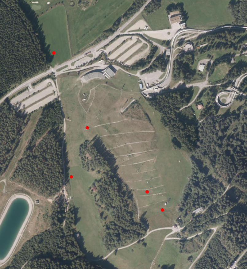
Study site

The study site at the base of Patscherkofel with the four measurement points (bottom) and the reference point (top) for green grass (see section 2.3).

Results

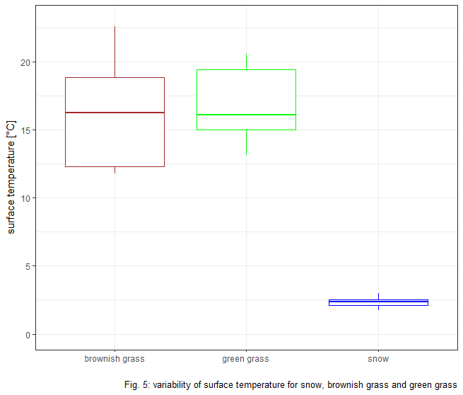
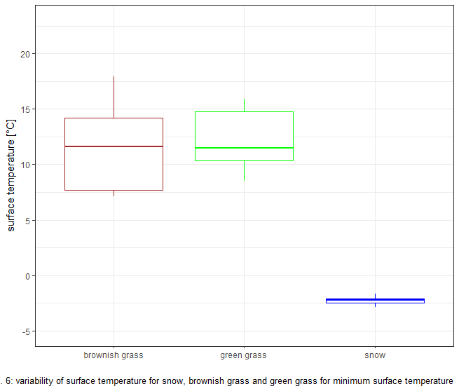
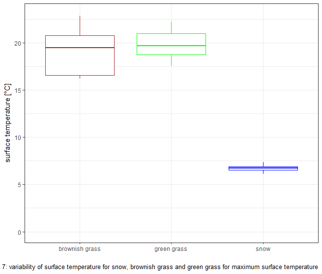
Albedo for snow,green and brownish grass

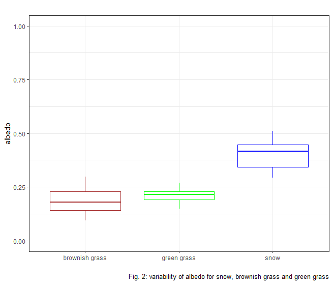
The boxplot shows the highest albedo values for snow and lowest albedo values for brownish gras. Within the upper range of brownish grass lies albedo range of green grass.

T-tests

We wish to determine the significance of differences in the mean albedo values between samples taken from three different populations (snow, green and brown grass). We assume the three distributions from which samples are taken are all Gaussian, but make no assumptions about their variances, or which populations have higher means. To compare the three populations, we split them into three pairs and perform a Welch Two Sample t-test for each population pair.

Welch Two Sample t-test

data:  g and b
t = 2.1221, df = 55.638, p-value = 0.0383
alternative hypothesis: true difference in means is not equal to 0
95 percent confidence interval:
 0.001351736 0.047044403
sample estimates:
mean of x mean of y
0.2088843 0.1846862


Welch Two Sample t-test

data:  g and s
t = -15.915, df = 53.002, p-value < 2.2e-16
alternative hypothesis: true difference in means is not equal to 0
95 percent confidence interval:
 -0.2169342 -0.1683748
sample estimates:
mean of x mean of y
0.2088843 0.4015388


Welch Two Sample t-test

data:  s and b
t = 14.8, df = 69.589, p-value < 2.2e-16
alternative hypothesis: true difference in means is not equal to 0
95 percent confidence interval:
 0.1876269 0.2460782
sample estimates:
mean of x mean of y
0.4015388 0.1846862

Our Null Hypothesis is that there is no difference in the means of the two distributions from which samples are taken. The test results give us a 95% confidence interval for the difference in means.

For green and brown grass, the 95% confidence interval for the difference in means is [0.0014,0.0470]. We are therefore 95% sure that the mean albedo of the distribution from which the green grass samples are taken is slightly higher than that of brown grass.

The 95% confidence interval for the difference in means between snow and green grass is [0.1683,0.2169]. We are therefore 97.5% sure that the mean snow albedo is at least 0.1683 greater than the mean green grass albedo.

For snow and brown grass the results are similar to snow and green grass. The 95% confidence interval is [0.1876,0.2461].

Albedo for snow, green and brownish grass; slope parallel and horizontally

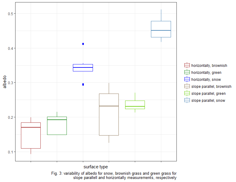
Horizontally measured, albedo values are overall smaller for snow, brownish and green grass, respectively.

NDVI & Albedo

The Normalized Difference Vegetation Index provides information about the state of living vegetation whereby higher values indicate greener grass.

NDVI is based on the reflection of green grass in the red and near infrared wavelength range.

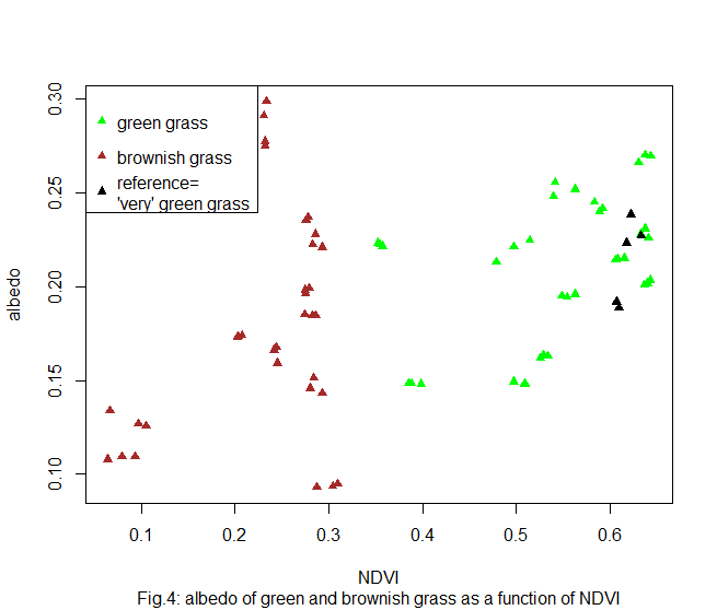
As expected, NDVI is higher for green grass and the reference (‘very’ green grass) compared to brownish grass.

Since green grass has slightly higher albedo values than brownish grass (See Fig. 2) and higher NDVI value, we would have expected higher albedo values with higher NDVI.

Due to high variability within the brownish grass, NDVI and albedo values reveal no apparent relation.

Derive Surface temperature from outgoing LW

From our 4-component radiometer we can not only investigate the short wave components of radiation (from the sun), but also the longer wavelengths emitted by significantly cooler bodies (such as the earth’s surface or clouds). From the Stefan-Boltzmann Law, we can estimate the surface temperature assuming the measured outgoing longwave radiation is exactly equal to the radiant emittance of the surface below the sensor. Furthermore we assume the temperature of the radiating body remains relatively constant over depths of similar magnitude to the optical depth.

The emissivity of snow and soil are both close to unity. Thus, we assume an emissivity of one in the following calculations and this means our derived surface temperatures are a lower limit.

Potential sources of error

Our snow surface temperature estimates are above freezing, which is something we do not expect. The following explanation could be the potential sources of error.

Calibration uncertainty & offset

Due to a Calibration Uncertainty of ± 5 % and a Zero Offset B value of less than 5 W/m$^2$ (https://www.apogeeinstruments.com/net-radiometer/), possible maximum and minimum surface temperatures were calculated:

The deviation from the freezing point lies within the calibration uncertainty and offset.

Influence of the observer

Another possible explanation of this phenomenon is that the observer holding the ecobot influences the outgoing longwave radiation measurement.

We wish to estimate this influence of longwave radiation emitted by the person holding the ecobot on the measurement (for flat ground). We know that the pyrgeometer has a directional cosine response and a field of view of 150$^\circ$. We define a weighting function $\delta = \delta(r) \propto \phi,$ where $\phi$ is the angle with respect to the normal line through sensor, that has the property $\int_{r=0}^{r=r_2} \int_{\theta=0}^{2\pi} \delta(r) r \,d\theta\,dr = 1$.

From simple trigonometric considerations, we see that $\delta (r) = \lambda \frac{h}{h^2+r^2},$ where h is the height of the pyrgeometer above ground and $\lambda$ is a constant which needs to be chosen such that the integral property above is fulfilled.

We find that $\lambda = \frac{1}{\pi h \ln(\frac{h^2+r_2^2}{h^2})},$ where $r_2$ is the distance from the surface point below the pyrgeometer to the intersection of the 150$^\circ$ width cone and the surface plane (it is the radius of the surface of influence).

We assume that the person holding the ecobot stands at a distance $r_1 = 1$ m from the pyrgeometer and has a width of $w = 0.3$ m. Then the angular width of the person is approximately $\theta_1 = w/r_1$.

The outgoing longwave radiation measured by the pyrgeometer can be expressed as the weighted integral of the longwave radiation emitted by the surface and the observer. We replace the surface longwave radiation in the region ‘blocked’ by the observer with that emitted by the observer themselves.

where we define $LW_{out}$ as constants $LW_b$ or $LW_s$ for the outgoing radiation emitted by the blocked and snowy regions respectively. Since $LW_{out}$ is a piecewise constant function, our problem becomes simpler and we only need to find the weighted fractional area blocked by our observer. This is given by

Given values of $\theta_1 = 0.3$, $h = 1$ m, $r_2 = 3.75$ m, and $r_1 = 1$ m, we arrive at an estimate for the weighted blocked area: $\delta_b \approx 0.036$.

Then $LW_{measured} = \delta_b LW_{b} + (1-\delta_b) LW_{s}$.

Assuming temperatures of $T_b = 40^{\circ}$C and $T_b = 0^{\circ}$C, our snow surface temperature (inferred from the measured longwave radiation) would be

We can also rearrange the previous relation of $LW_{measured}$, $LW_b$ and $LW_s$ to arrive at the minimum blocking fraction required to explain the error in our surface temperature estimate:

Substituting the appropriate values, we arrive at $\delta_{b}^{crit} \approx 0.05$ By changing the width (along the circle of radius $r_1$) of the blocking observer to 0.5 m, $\delta_b$ increases to 0.059 and $\hat{T} = 276.05 \textrm{K} \approx 2.9^{\circ} \textrm{C}$.

It seems like the influence of the human observer can explain our unexpectedly high snow surface temperature estimates quite well.

Water film

Another explanation for the higher surface temperature of snow could be a thin water film formed by snowmelt. This liquid water could influence the estimated surface temperature to varying magnitudes, depending on the relationship between the film thickness and the optical depth of water for thermal wavelengths.

Reflected Longwave Radiation

Our assumption in using outgoing longwave radiation measurements to estimate surface temperature is that all of the measured radiation is emitted by the surface. The fraction of downgoing longwave radiation reflected by the surface is $1-\alpha$ where $\alpha$ is the average (weighted) albedo over thermal wavelengths.

Instead of just using the outgoing longwave radiation to derive the surface temperature assuming an emissivity of one, we can use our measured incoming longwave radiation along with knowledge of the surface emissivity to arrive at a better estimate.

In the case where $LW_{in} = LW_{out}$, our assumption works perfectly. The outgoing measured radiation is related to the surface temperature with an emissivity of one. This condition may be close to fulfilled in cloudy or especially foggy conditions.

In the case where $LW_{in} = 0$, no longwave radiation is reflected at the surface and we need to correct our outgoing measurement with the proper surface emissivity.

For our case, the two approaches reveal the difference of approximately 1.5°C. Assuming an emissivity of 1 gives the lowes surface temperature estimate.

Discussion

Let us consider the significance of this albedo difference between snow and no-snow surfaces on a slope with artificial vs. natural snow cover. The effect of the albedo is, of course, directly proportional to the magnitude of the incoming solar radiation. If there is little incoming solar radiation, the difference in the radiative balance is not large even for very different surface albedos. Let us try to estimate the maximum direct radiative influence of artifical snow making at a large scale.

In the extreme case, there is no natural snow and only artificial snow on the mountain for four months of the year. If we assume that all slopes receive the maximum possible incoming solar radiation $S_{max}$, the difference in absorbed shortwave radiation while the sun is shining on snow compared to grass is $S_{max} \alpha_{\Delta}$. But, this difference is just while the sun is shining and for the ski resort area. On a larger scale, we would also need the area of all ski resorts as a fraction of the total Austrian area. There are approximately 400 ski areas in Austria. Assume an average ski resort has 50 km piste with an average width of 50 m. Then all Austrian ski resorts have an area of 1000 km$^2$ which is approximately 1% of the total Austrian area. This is surely a very high estimate.

The average shortwave radiative forcing on an Austrian scale would then be

Substituting values of 500 W/m$^2$ for $S_{max}$ and 0.2 for $\alpha_{\Delta}$, we arrive at a maximum radiative forcing estimate for artificial snow (at the Austrian scale) of slightly less than 1 W/m$^2$. For comparison, this is about half the magnitude of the radiative forcing of carbon dioxide (at a global scale) when compared to pre-industrial levels.

But our estimated maximum value is at an Austrian scale and there are hardly many countries with such a high density of ski resorts. There are approximately 5000 ski areas in the world. Assuming they have similar size to the Austrian ski resorts, 1/10th of the world’s ski area is in Austria, while Austria is only 1/5000th of the world’s area.

Then we have a radiative forcing estimate of artifical snowmaking for the whole earth of approximately 1/500 W/m$^2$ which seems more reasonable when compared to carbon dioxide.

This estimate neglects any effects apart from direct influences on the short-wave budget. Snowpack additionally emits less longwave radiation in the spring melt season compared to grassland. This would counter the albedo effect and cause less energy loss for the surface. Turbulent heat fluxes can also be suppressed due to more stable stratification above the snow surface. Therefore our estimate of the radiative forcing should be seen as an absolute maximum order-of-magnitude estimate.