from IPython.display import HTML
HTML('''<script>
code_show=true;
function code_toggle() {
 if (code_show){
 $('div.input').hide();
 } else {
 $('div.input').show();
 }
 code_show = !code_show
}
$( document ).ready(code_toggle);
</script>
The raw code for this IPython notebook is by default hidden for easier reading.
To toggle on/off the raw code, click <a href="javascript:code_toggle()">here</a>.''')
Analysis of the Albedo in transition between snow and no snow in Neustift
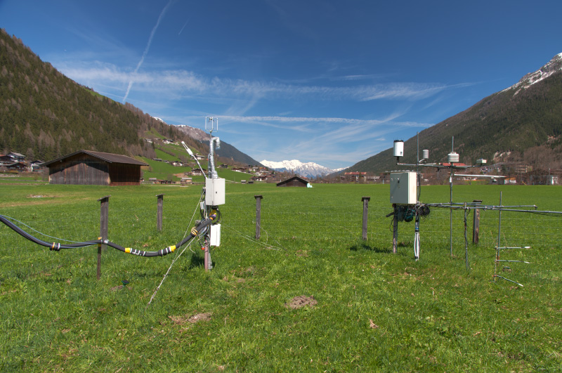 Automatic Weather Station Neustift
Picture taken from http://www.biomet.co.at/research/field-sites/neustift-austria/
In our investigation of the effects of artifical snow on the radiative forcing the change of the surface albedo caused by the prolonged existence of snow-cover on the skiing slopes is the most prominent negative one.
To investigate the differences between the albedo of snow-cover and no snow-cover,data from the weather station in Neustift (Stubaital) was investigated.
The available data spans over a time-period from 2010 to 2017. In those years especially the transition time from snow to no-snow conditions is interesting.
%matplotlib inline

import matplotlib.pyplot as plt  # plotting library
import matplotlib.dates as mdates
import numpy as np  # numerical library
import xarray as xr  # netCDF library
import pandas as pd
from datetime import datetime
import warnings
warnings.filterwarnings('ignore')

import cufflinks as cf
import plotly
import plotly.offline as py
import plotly.graph_objs as go
from plotly import tools
init_notebook_mode(connected=True)

cf.go_offline() # required to use plotly offline (no account required).
data_neustift = pd.read_excel(io = './data/dataGeorgWohlfahrt_Neustift.xlsx', sheet_name = None, skiprows=[1], parse_dates = True, index_col = 0)
year_array = ['2010', '2011', '2012', '2013', '2014', '2015', '2016', '2017']
dates = pd.date_range(start='01-01-2010', end='31-12-2017')
# Calculate Albedo-values, values with an incoming shortwave radiation smaller than 50 Wm-2
# or an calculated Albedo above 1 are ignored

for i in range(0,len(year_array)):

    data_neustift[year_array[i]]['Albedo'] = data_neustift[year_array[i]].SW_out / data_neustift[year_array[i]].SW_in
    data_neustift[year_array[i]]['Albedo'] = np.where(np.logical_or(data_neustift[year_array[i]]['SW_in'] < 50, data_neustift[year_array[i]]['Albedo'] > 1), np.nan, data_neustift[year_array[i]]['Albedo'])
    data_neustift[year_array[i]]['SNOWH'] = data_neustift[year_array[i]]['SNOWH'].where(data_neustift[year_array[i]]['SNOWH'] < 1.64)
# Function to calculate daily average Albedo-values
# The daily average albedo is taken as the sum of reflected radition divided by the sum of the incoming radiation

def daily_avg_albedo(year):
    swin = data_neustift[str(year)].SW_in
    swout = data_neustift[str(year)].SW_out
    daily_avg_albedo = swout.resample('D').sum() / swin.resample('D').sum()
    return daily_avg_albedo


# Calculating daily average albedo-values for all the years.
# Data is stored in dictionary. To access for example the results for 2017 use:
# albedo_avg_dict['2017']

albedo_avg_dict = {}
snowh_avg_dict = {}
for i in range(0,len(year_array)):
    albedo_avg_dict[year_array[i]] = daily_avg_albedo(year_array[i])
    #albedo_avg_dict[year_array[i]] = np.where(albedo_avg_dict[year_array[i]] > 1, np.nan, albedo_avg_dict[year_array[i]])
    albedo_avg_dict[year_array[i]] = albedo_avg_dict[year_array[i]].where(albedo_avg_dict[year_array[i]] < 1)
    snowh_avg_dict[year_array[i]] = data_neustift[year_array[i]].SNOWH.resample('D').mean()
## Concentate albedo values to get one array for the whole period
albedo_all_years = albedo_avg_dict[year_array[0]]
snowh_all_years = snowh_avg_dict[year_array[0]]
for i in range(1,len(year_array)):
    albedo_all_years = np.append(albedo_all_years,albedo_avg_dict[year_array[i]])
    snowh_all_years = np.append(snowh_all_years, snowh_avg_dict[year_array[i]])

df_alb_snowh = pd.DataFrame([dates, albedo_all_years, snowh_all_years]).transpose()
df_alb_snowh.rename(columns={0:'Dates', 1:'Albedo', 2:'Snowh'}, inplace = True)
df_alb_snowh.set_index('Dates', inplace = True)
df_alb_snowh['Albedo'] = pd.to_numeric(df_alb_snowh.Albedo, errors = 'coerce')
df_alb_snowh['Snowh'] = pd.to_numeric(df_alb_snowh.Snowh, errors = 'coerce')
def transition_albedo(year):
    transition_albedo = albedo_avg_dict[str(year)].loc[str(year)+'-01-01': str(year)+'-04-30']
    return transition_albedo

def transition_snowh(year):
    transition_snowh = data_neustift[str(year)].SNOWH.loc[str(year)+'-01-01': str(year)+'-04-30']
    return transition_snowh
albedo_trans_dict = {}
snowh_trans_dict = {}

for i in range(0,len(year_array)):
    albedo_trans_dict[year_array[i]] = transition_albedo(year_array[i])
    snowh_trans_dict[year_array[i]] = transition_snowh(year_array[i])
color1 = '#1f77b4'
color2 = 'grey'

trace2 = go.Bar(
    x = df_alb_snowh.index,
    y = df_alb_snowh.Snowh,
    name='Snowheight',
    yaxis='y2',
    opacity = 0.5,
    marker = dict(
        line = dict(
            color = color2),
        color = color2)
)

trace1 = go.Scatter(
    x = df_alb_snowh.index,
    y = df_alb_snowh.Albedo,
    name = 'Albedo',
    line = dict(
        color = color1
    )
)

data = [trace1, trace2]
layout = go.Layout(
    title= "Albedo and Snowheight over the whole period",
    yaxis=dict(
        title='Albedo',
        range = [0,1],
        gridcolor = 'white',
        titlefont=dict(
            color=color1
        ),
        tickfont=dict(
            color=color1
        )
    ),
    yaxis2=dict(
        title='Snow-Height',
        range = [0,1],
        gridcolor = 'white',
        overlaying='y',
        side='right',
        titlefont=dict(
            color=color2
        ),
        tickfont=dict(
            color=color2
        )

    )

)
fig = go.Figure(data=data, layout=layout)
plot_url = py.iplot(fig)
In the plot above you can see the daily average albedo and the measured snow-height for the whole eight years of available data. Already in this plot it's easy to see that there is a big difference in the albedo-values between summer in winter. For all years the albedo in summer is quite constant with values a bit above 0.2. In winter the albedo is stronger fluctuating but is mostly in a range between 0.7 and 1.
The positive snow-height measurements in summer are caused by the lawn under the sensor. The sensor is just measuring the distance to the ground and can't see if the ground is snow or grass. When the snow-height measurements suddenly drop in summer it's a sign that the grass was cut. It's interesting to see that with cutting the grass the albedo also drops.
To get an better idea how the albedo is behaving when the snow melts in spring in the following the time from January until the end of April for each year is investigated more precisely.
trace_dict = {}

trace_dict['0'] = go.Scatter(
    x = albedo_trans_dict[year_array[0]].index,
    y = albedo_trans_dict[year_array[0]],
    name = 'Albedo',
    line = dict(
        color = color1
    )
)

trace_dict['1'] = go.Bar(
    x = snowh_trans_dict[year_array[0]].index,
    y = snowh_trans_dict[year_array[0]],
    name = 'Snowheight',
    opacity = 0.5,
    marker = dict(
        line = dict(
            color = color2),
        color = color2)
)

for i in range(2,2*len(year_array),2):
    trace_dict[str(i)] = go.Scatter(
        x = albedo_trans_dict[year_array[int(i/2)]].index,
        y = albedo_trans_dict[year_array[int(i/2)]],
        name = 'Albedo',
        showlegend = False,
        line = dict(
            color = color1
        )
    )

    trace_dict[str(i+1)] = go.Bar(
        x = snowh_trans_dict[year_array[int(i/2)]].index,
        y = snowh_trans_dict[year_array[int(i/2)]],
        name = 'Snowheight',
        showlegend = False,
        opacity = 0.5,
        marker = dict(
            line = dict(
                color = color2),
            color = color2)
    )
y_axis = ['yaxis1', 'yaxis2', 'yaxis3', 'yaxis4', 'yaxis5', 'yaxis6', 'yaxis7', 'yaxis8']
x_axis = ['xaxis1', 'xaxis2', 'xaxis3', 'xaxis4', 'xaxis5', 'xaxis6', 'xaxis7', 'xaxis8']
labels = ['Jan', 'Feb', 'Mar', 'Apr', 'May']

fig = tools.make_subplots(rows = 4, cols = 2, subplot_titles=year_array)
for i in range(0, len(trace_dict),4):
    fig.append_trace(trace_dict[str(i)], int(i/4)+1, 1)
    fig.append_trace(trace_dict[str(i+1)], int(i/4)+1, 1)
    fig.append_trace(trace_dict[str(i+2)], int(i/4)+1, 2)
    fig.append_trace(trace_dict[str(i+3)], int(i/4)+1, 2)

fig['layout'].update(height = 1500, title='Albedo and snow-height from January to May')
for y in y_axis:
    fig['layout'][y].update(range=[0,1], dtick = 0.2)

i = 0
for x in x_axis:
    fig['layout'][x].update(tickvals = (pd.to_datetime(['01-01-'+year_array[i], '01-02-'+year_array[i], '01-03-'+year_array[i], '01-04-'+year_array[i], '01-05-'+year_array[i]], format = '%d-%m-%Y')), ticktext = labels, ticklen = 4, tickwidth = 1)
    i = i+1

py.iplot(fig, filename='transition_period')
In all years it's clearly visible that there is a time in spring, when the Albedo reaches a value of about 0.2 and stays fairly constant. The attainment of this value is accompanied with a local minima in the snow-height. This indicates the point when the snow is gone and the grass starts growing. So we can conclude that the Albedo of grass is about 0.2. Seperate spikes after the Albedo had already reached it's value for grass are caused by snowfall and the resulting snowcover.
When there is a snow-cover the Albedo-value is not as constant as for grass. It varies between values of above 0.9 for fresh snow and an value of 0.6 for old snow. Compared with the snow-height values we can see, that the Albedo goes up after snow-fall and decreases the older the snow on top of the snow-cover gets. It's also decreasing when the snow-cover starts to melt.
The transition between snow-albedo and grass-albedo happens in a matter of days in each year. The decrease in the Albedo before the snow is totally gone is caused by a film of meltwater on top of the snow or by a mix of snow- and grass-albedo caused by patches where the snow is already gone.
- The effect of the decreasing Albedo with age of the snow can nicely be observed in 2011. Between the middle of January and the middle of February the snow-height is fairly constant and the Albedo is slowely decresing.
- The effect of snowfall after the snow-cover was already melted can be seen in several years, for example in 2014 with snowfall in the end of March and a change in the Albedo from about 0.2 to about 0.9.
- The strong sparkes in the snow-height sensor to values higher than 1m, mostly pronounced in 2010 and 2013 could are false measurements. They could be caused by really strong fog or snowfall, so the sensor can't 'look' to the ground anymore.